

Heterogeneous Decentralized Diffusion Models
Training-free merging of diffusion experts trained with different objectives


Based on Bagel Labs' CVPR 2026 paper on Heterogeneous Decentralized Diffusion Models: arxiv link
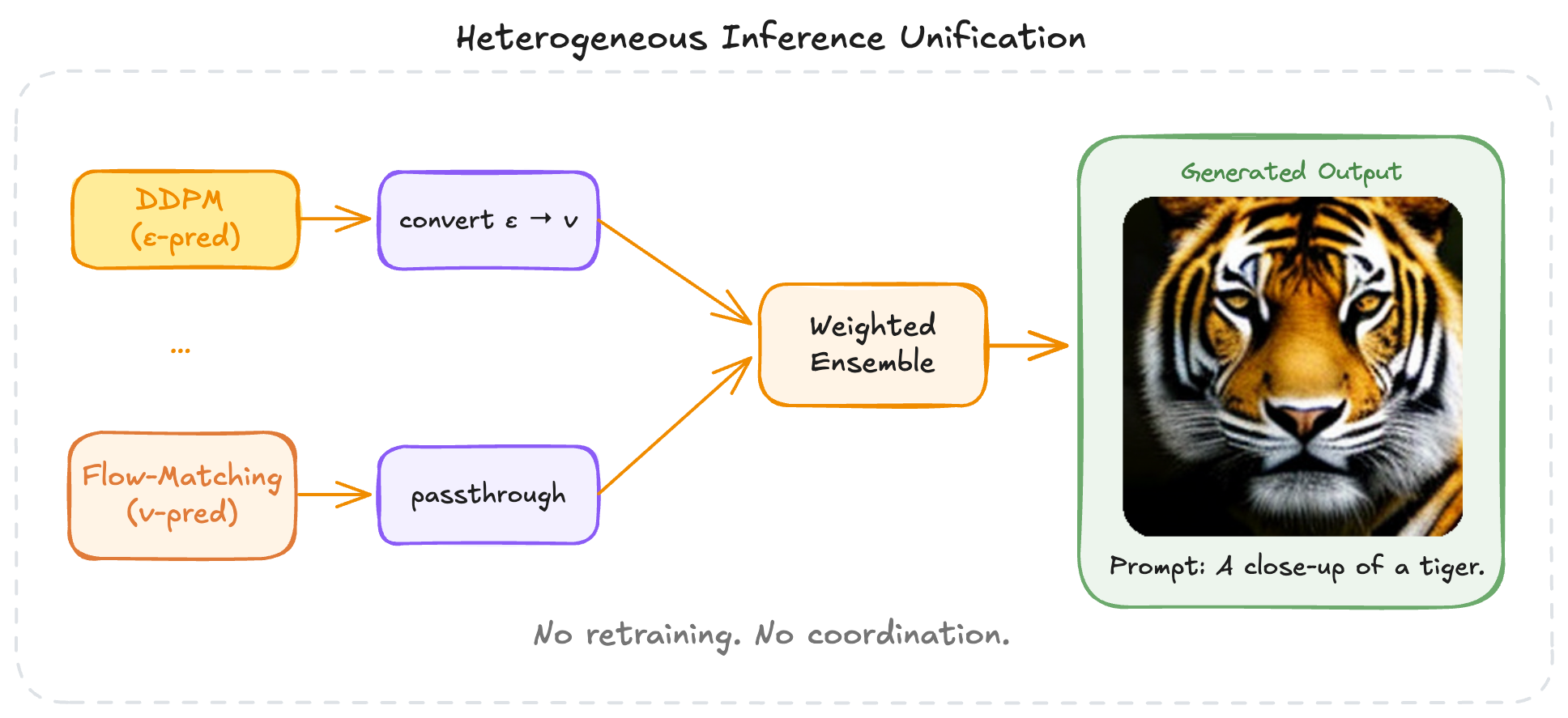
Decentralized Diffusion Models (DDMs) train independent experts on disjoint data partitions and combine them at inference time. Existing DDM frameworks assume all experts share the same training objective. We relax this constraint. In our setup, some experts train with DDPM (ε-prediction) and others with Flow Matching (velocity-prediction), then unify at inference through a deterministic conversion into a common velocity space. No retraining, no fine-tuning, no coordination during training.
Heterogeneous experts trained independently on single GPUs, unified at inference through velocity conversion.
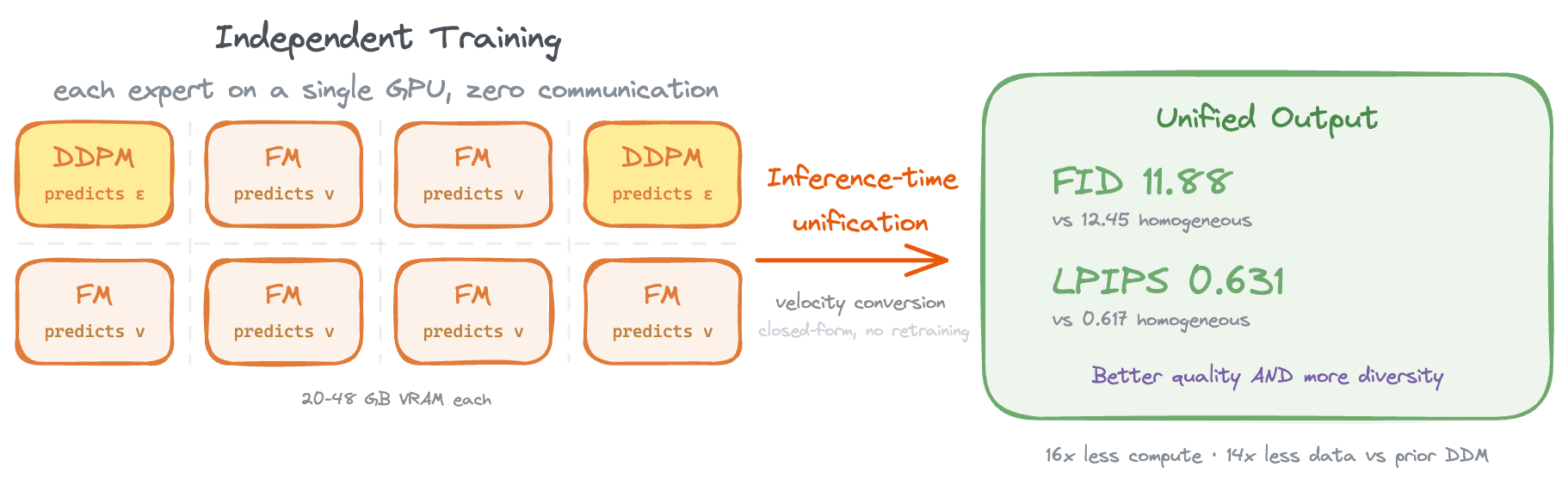
Under aligned inference settings, this heterogeneous ensemble (2 DDPM + 6 FM experts) achieves better FID (11.88 vs. 12.45) and higher intra-prompt diversity (LPIPS 0.631 vs. 0.617) than a homogeneous ensemble of 8 FM experts. Relative to the training scale reported for prior DDM work, our framework reduces compute from 1176 to 72 A100-days (16×) and data from 158M to 11M images (14×), with each expert requiring only 24–48 GB VRAM on a single GPU, making decentralized diffusion training accessible on commodity hardware.
Background: Decentralized Flow Matching
DDMs decompose a generative model into K experts, each trained on a semantically coherent subset of the data. Following prior DDM work, the marginal velocity field is expressed as a weighted combination of per-expert conditional flows:
where uₜ⁽ᵏ⁾(xₜ) is the velocity predicted by expert k trained on cluster Sₖ, and pₜ(k | xₜ) is a posterior weight from a learned router.
Training
We partition the dataset into K semantic clusters using DINOv2 features (1024-dimensional representations with hierarchical k-means). This produces semantically coherent partitions, e.g. portraits, landscapes, architecture. Each expert θₖ trains exclusively on its assigned cluster Sₖ with zero communication between experts. No shared parameters, no gradient synchronization, no activation passing.
Routing
A lightweight router (DiT-B, 129M parameters) learns to predict cluster assignments from noisy inputs:
trained with cross-entropy loss against ground-truth cluster labels. At inference, the router dynamically selects and weights experts based on the current noisy state and timestep. We support three selection modes: Top-1 (single best expert), Top-K (weighted ensemble of K highest-probability experts), and Full Ensemble (all experts weighted by router probabilities). As shown in our prior work, Top-2 routing consistently outperforms Full Ensemble because sparse routing maintains expert-data alignment, selecting experts that are in-distribution for the current denoising state.
Heterogeneous Objectives
Previous DDM work requires all experts to share the same training objective. This is a coordination requirement that may be impractical when contributors operate independently. We remove this constraint.
Two objectives, different emphasis
We train n experts with Flow Matching loss and m experts with DDPM loss. DDPM experts predict the noise ε added during the forward process:
Flow Matching experts predict the velocity field directly:
Here x₀ ∈ Sₖ means expert k trains only on clean samples from its assigned cluster Sₖ, ε ~ N(0, I) is Gaussian noise, t is the sampled timestep, and αₜ, σₜ are the schedule coefficients controlling signal and noise strength, xₜ = (1-t)x₀ + tε is the linear interpolation between clean data and noise.
Both objectives model the same generative process through different parameterizations. But they weigh errors differently across timesteps, and this difference is the mechanism behind heterogeneous ensembles.
Complementary loss weighting
We can write both losses in terms of the squared clean-sample estimation error |x̂₀ - x₀|² (the detailed derivation can be read from variational diffusion models). Under a variance-preserving schedule (αₜ² + σₜ² = 1):
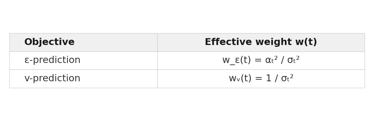
The ratio between them is:
Here w_ε(t) and wᵥ(t) are the effective per-timestep weights after rewriting each loss in terms of clean-sample estimation error. Since αₜ ≤ 1 and decays toward 0 at high noise, this ratio diverges. Velocity-prediction experts receive relatively stronger gradients at high-noise timesteps (global structure), while ε-prediction experts are relatively upweighted at low noise (fine details). In the paper, we derive this under a variance-preserving schedule and then note that linear interpolation recovers the same 1 / αₜ² structure. So the complementary weighting pattern holds both for the VP analysis and for the linear FM path used here.
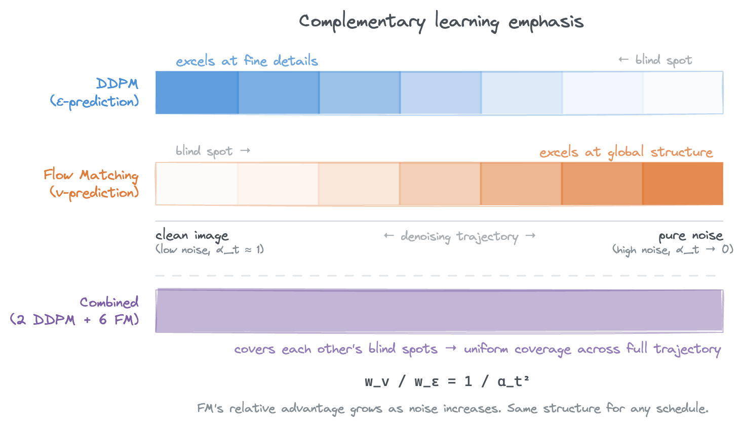
DDPM concentrates learning signal near clean images. Flow Matching emphasizes high-noise timesteps. Their blind spots are complementary.
The implication is that each objective has a “blind spot” region where its effective weight is relatively low, and these blind spots are complementary. Where DDPM under-trains (high noise), FM trains hardest. Where FM under-trains (low noise), DDPM concentrates its signal. Mixing both in an ensemble lets each objective cover the other’s blind spots, providing more uniform coverage across the full denoising trajectory.
Inference-Time Unification
The central technical challenge is that DDPM experts output noise predictions ε_θ(xₜ, t) while FM experts output velocity predictions v_θ(xₜ, t). These live in different spaces. You cannot average them directly.
We unify all expert predictions into a common velocity space through a deterministic, schedule-aware conversion. The derivation proceeds in three steps.
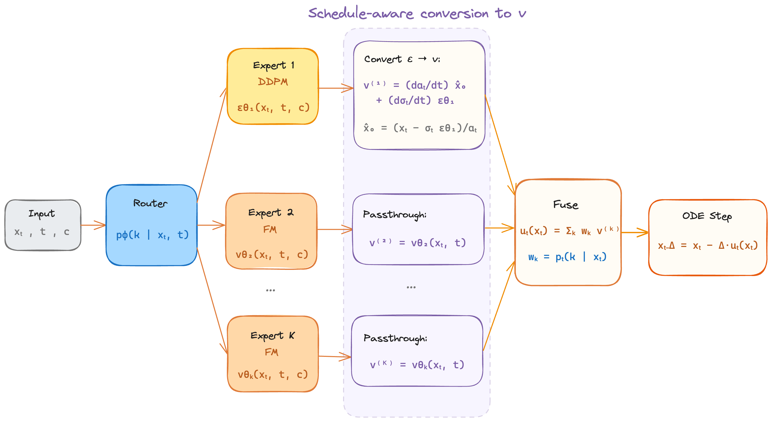
The conversion pipeline: DDPM noise predictions are converted to velocity through deterministic algebra. FM predictions pass through unchanged.
Step 1: Recover the clean-image estimate
From the DDPM forward process xₜ = αₜ x₀ + σₜ ε, invert the linear map using the model’s noise prediction:
Step 2: Derive the velocity
Treating x̂₀ and ε_θ as fixed at their current-timestep values defines a deterministic path x̃ₜ = αₜ x̂₀ + σₜ ε_θ. Differentiating with respect to t:
Under linear interpolation (αₜ = 1-t, σₜ = t), the schedule derivatives are -1 and +1, so this simplifies to:
This is exactly the FM velocity target v = ε - x₀.
Step 3: Combine
FM experts already output velocity, so they pass through unchanged. All predictions are now in the same space. The router assigns per-expert weights, and we take a weighted combination to form the ensemble field uₜ, which drives a standard ODE integration step (x_{t−Δt} = xₜ − uₜ · Δt).
Numerical stability
The conversion requires dividing by αₜ, which approaches zero at high noise. We apply three safeguards: (1) clamp x̂₀ to [-20, 20] for VAE latents, (2) use α_safe = max(αₜ, 0.01) in the denominator, and (3) apply adaptive velocity scaling that dampens converted predictions at elevated noise levels where schedule derivatives become large. These are simple clamps with no learned parameters.
The entire conversion is closed-form algebra. No learned components, no fine-tuning, no additional training of any kind.
Efficient Training
Prior DDM work required 1176 A100-days on 158M images. We achieve competitive quality with 72 A100-days on 11M images, a 16× reduction in compute and 14× in data. Three techniques enable this.
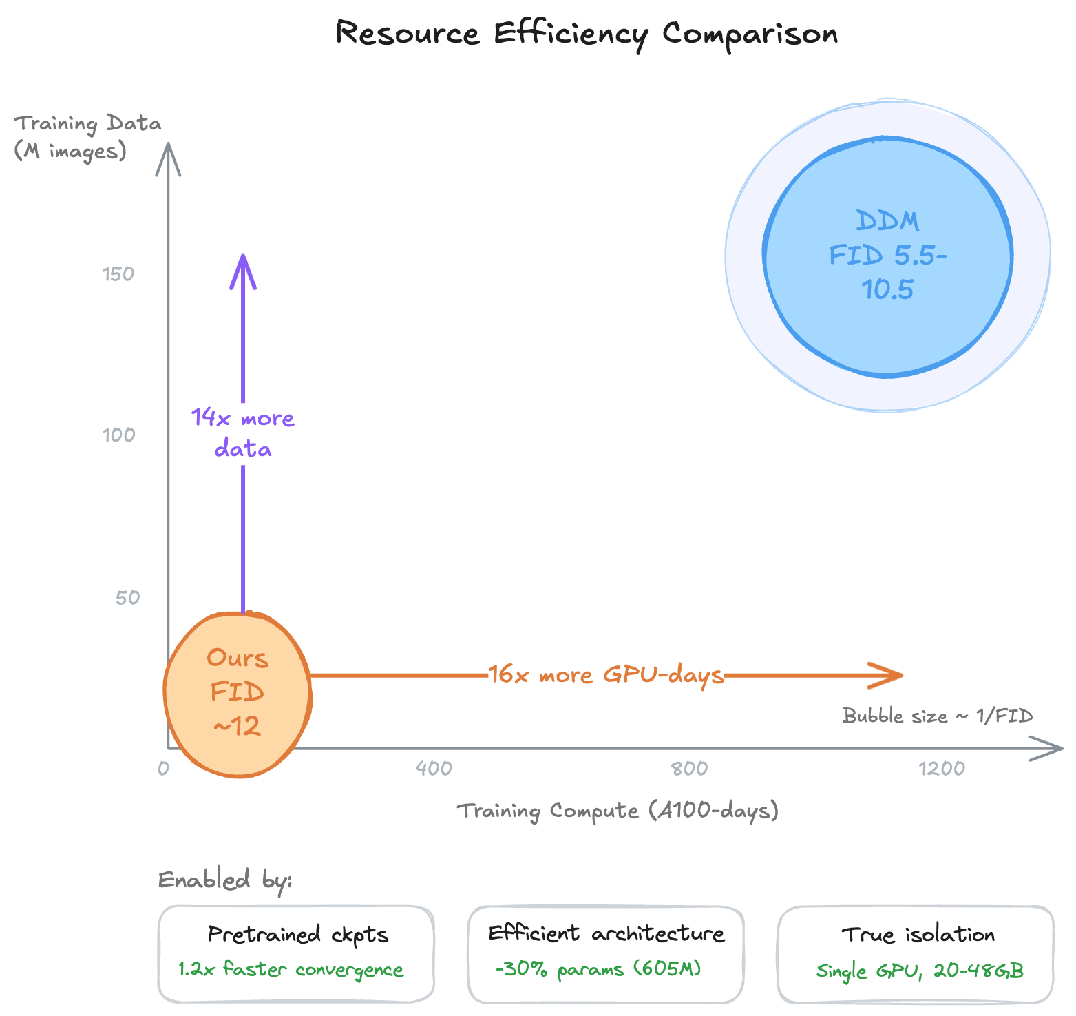
Resource comparison: our approach requires a fraction of the compute and data of prior DDM work.
Pretrained checkpoint conversion
We initialize experts from ImageNet-pretrained DiT checkpoints. Patch embeddings, positional embeddings, and all transformer blocks are fully transferred. Only the final projection layer (which differs between ε- and velocity-prediction targets) and the text projection (new modality) are reinitialized. Class-conditional embeddings from ImageNet pretraining are removed.
A key technical detail is timestep compatibility. DiT models expect discrete timesteps t ∈ {0, 1, …, 999} while Flow Matching uses continuous t ∈ [0, 1]. We handle this with runtime conversion (t_DiT = round(999t)) rather than modifying pretrained weights, preserving the learned timestep embedding structure.
Converted checkpoints reach validation loss parity 1.2× faster than training from scratch.
Efficient architecture
Each expert uses DiT with PixArt-α’s AdaLN-Single conditioning. Rather than computing adaptive layer normalization parameters with per-block MLPs, a single global MLP produces all modulation signals:
reshaped into per-block slices plus learned per-block embeddings Eᵦ. This reduces parameters by 30% (891M to 605M for DiT-XL/2) while maintaining generation quality.
True isolation
Each expert trains on its own semantic cluster on a single GPU requiring 20–48GB VRAM. No gradient synchronization, no activation passing, no pipeline coordination, no parameter servers. This is not data parallelism with relaxed communication. There is literally zero inter-expert communication during training.
Experiments
We train on 11M LAION-Aesthetics images. For a high-quality subset of 3.9M images, we use LLaVA to generate improved captions. We evaluate using FID-50K on a held-out 50K test set. We train at two scales: DiT-B/2 (129M parameters per expert) and DiT-XL/2 (605M parameters per expert).
Our standard configuration uses K=8 experts. Experts 0 and 3 train with DDPM objectives (assigned to clusters containing high-fidelity subjects where ε-prediction excels at detail preservation). The remaining six use Flow Matching.
Monolithic versus decentralized
We first validate that decentralized training works. Using DiT-B/2 experts trained from scratch on LAION-Art (3.9M images), all with Flow Matching:
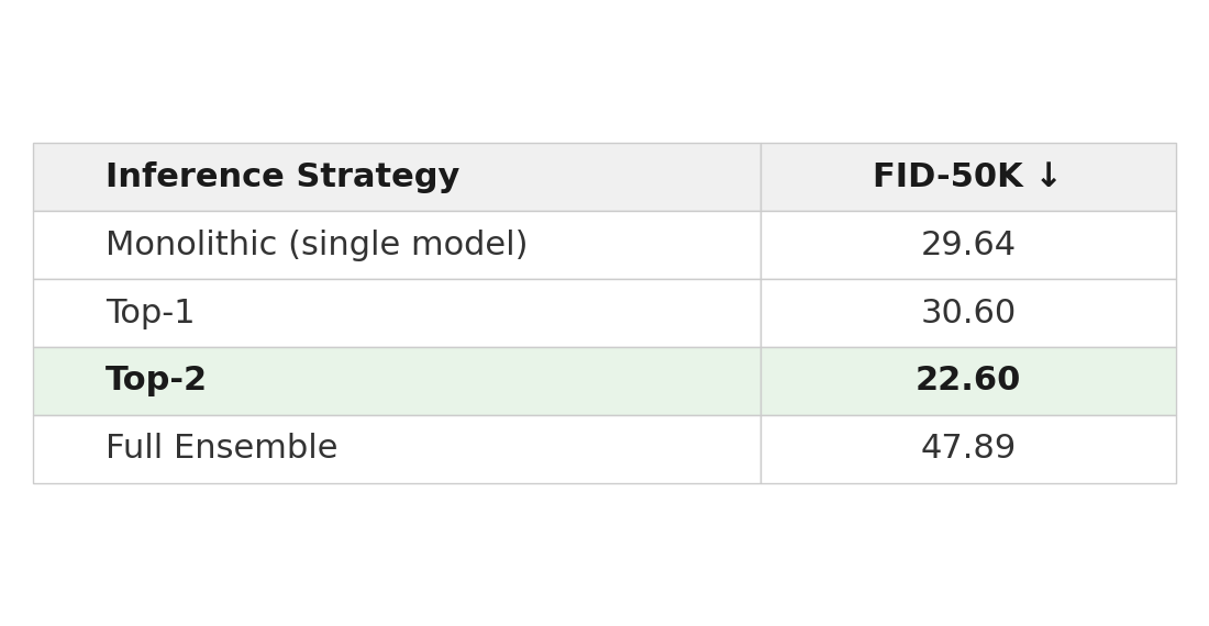
Top-2 achieves 22.60, outperforming the monolithic baseline by 23.7%. Full Ensemble underperforms dramatically (47.89), consistent with our prior finding that indiscriminate combination introduces prediction conflicts from out-of-distribution experts. Selective expert activation is essential.
Homogeneous versus heterogeneous
To isolate the effect of objective heterogeneity, we compare homogeneous and heterogeneous 8-expert DiT-XL/2 models under matched inference settings.
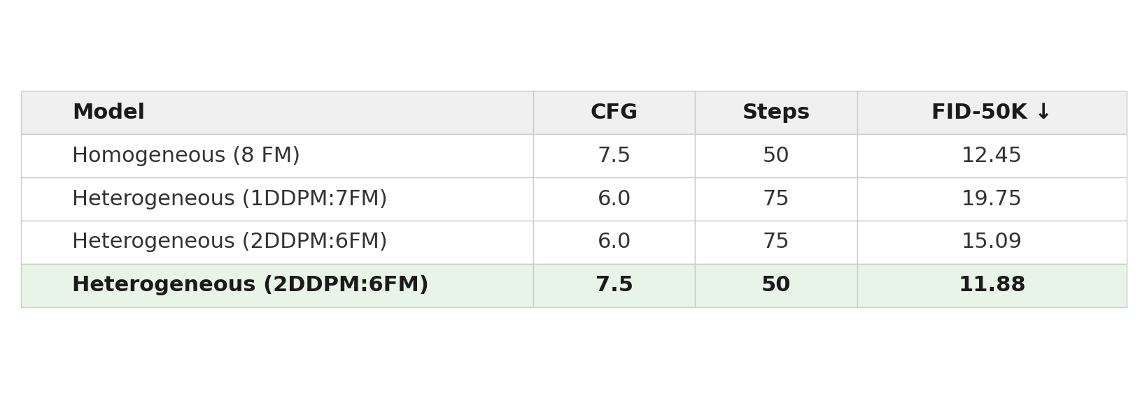
Under aligned settings (first and last rows), heterogeneous experts improve FID from 12.45 to 11.88. Scaling from 1 to 2 DDPM experts improves FID from 19.75 to 15.09 under the conversion setting, suggesting the optimal DDPM:FM ratio deserves careful tuning per domain.
For diversity, we measure intra-prompt LPIPS by generating 10 images per prompt for 100 held-out prompts. Heterogeneous experts achieve 0.631 (± 0.078) vs. homogeneous 0.617 (± 0.074). Objective heterogeneity produces more varied outputs for identical prompts.
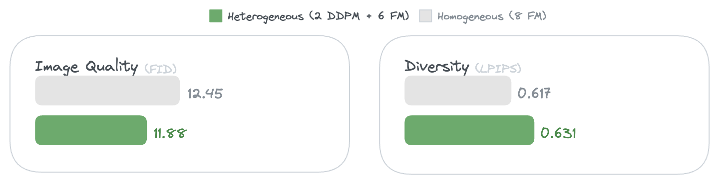
Heterogeneous ensembles improve both image quality (lower FID) and output diversity (higher LPIPS) over homogeneous baselines.
Conversion quality
We evaluate the DDPM → FM conversion in isolation, using experts trained on the same data cluster (to isolate objective effects from data distribution differences). Both DDPM and FM experts use DiT-XL/2 with identical hyperparameters.

Three findings emerge. First, the conversion works. DDPM → FM improves over native DDPM (FID 25.61 vs. 27.04) while preserving semantic coherence (CLIP 0.319 vs. 0.316). The conversion is most valuable as a compatibility mechanism rather than a lossless objective replacement.
Second, combined experts achieve higher output diversity (LPIPS 0.782) than single FM (0.752), approaching native DDPM levels (0.787). Heterogeneous objectives create complementary generation patterns.
Third, using the same cosine schedule for both objectives yields marginally better FID than different schedules (32.67 vs. 33.29), suggesting schedule alignment facilitates smoother expert transitions. But both combinations show similar diversity gains, indicating that objective heterogeneity drives the primary benefit.
Routing threshold analysis
For combined DDPM+FM experts, a deterministic router switches between them at a threshold t: DDPM handles timesteps t’ ≤ t (low noise), FM handles t’ > t (high noise).
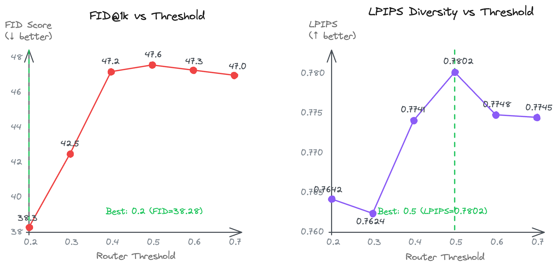
Impact of router threshold on generation quality. Different thresholds produce a clear quality-diversity trade-off.
Lower thresholds (0.2–0.3) favor quality (FM-dominated denoising, optimal FID). Mid-range thresholds (0.4–0.5) favor diversity (balanced workload, highest LPIPS). Extreme thresholds (0.7) degrade both metrics, confirming that both expert types contribute essential complementary capabilities.
Effects of expert ordering and router thresholds
Expert ordering also matters. In a 2-expert setup (1 converted DDPM + 1 FM), we vary the ordering — DDPM→FM versus FM→DDPM — and the switching threshold τ ∈ {0.3, 0.5, 0.7}.
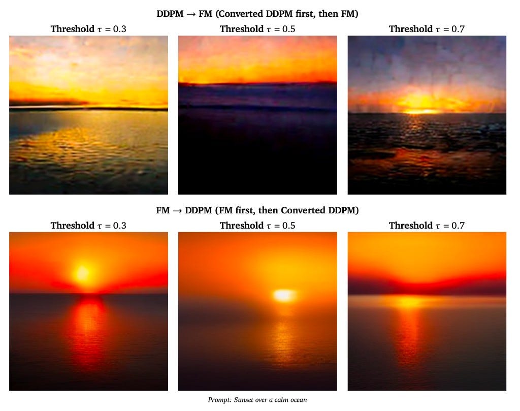
Expert ordering and router threshold effects. FM→DDPM ordering produces more stable, coherent results, while DDPM→FM shows higher sensitivity to threshold selection.
The results reveal a striking asymmetry. FM→DDPM (bottom row) produces consistently cleaner images across all thresholds. DDPM→FM (top row) degrades at higher thresholds, with blocky artifacts and oversaturation. The reason: when DDPM operates first at high noise (αₜ → 0), the conversion x̂₀ = (xₜ - σₜ ε_θ)/αₜ is numerically unstable, and errors early in the trajectory get baked into the image structure. Letting FM handle high-noise timesteps first avoids this entirely — the converted DDPM expert then refines at low noise where conversion is stable.
Takeaway: DDPM-to-velocity conversion should be restricted to low-noise regimes (t < 0.5).
Discussion
Resource efficiency in context
Our results should be interpreted carefully relative to prior DDM work. The DDM FID range of 5.5–10.5 was achieved at substantially larger training scale (1176 A100-days, 158M images). Our numbers are not directly comparable in absolute FID terms. What they do show is that competitive generation quality is attainable at a fraction of the resources, and that heterogeneous objectives provide an additional quality gain at no extra training cost.
Limitations
We evaluate only a narrow set of DDPM-to-FM ratios (1:7 and 2:6). The ideal allocation likely depends on the data distribution and downstream requirements. The deterministic conversion relies on hand-tuned numerical safeguards; a more robust conversion mechanism that generalizes across arbitrary schedules would strengthen applicability. We consider only ε- and velocity-prediction; extending to x₀-prediction or consistency objectives could further diversify expert specialization but would require generalizing the conversion and routing mechanisms.
What this enables
The practical upshot is that decentralized diffusion training no longer requires coordinated infrastructure or agreement on training objectives. A contributor with a single GPU can train a DDPM expert on portraits. Another can train an FM expert on landscapes using different hardware. These experts combine at inference time without either contributor needing to know what the other was doing.
Citation
@inproceedings{jiang2026heterogeneous,
  title     = {Heterogeneous Decentralized Diffusion Models},
  author    = {Jiang, Zhiying and Seraj, Raihan and Villagra, Marcos and Roy, Bidhan},
  journal = {arXiv preprint arXiv:2603.06741},
  year    = {2026}
}
congrats